Poisson Regression

import numpy as np
import matplotlib.pyplot as plt
import vowpalwabbit

%matplotlib inline

# Generate some count data that has poisson distribution
# z ~ poisson(x + y), x \in [0,10), y \in [0,10)
x = np.random.choice(range(0, 10), 100)
y = np.random.choice(range(0, 10), 100)
z = np.random.poisson(x + y)

We will model this data in two ways

• log transform the labels and use linear prediction (square loss)

• model it directly using poisson loss

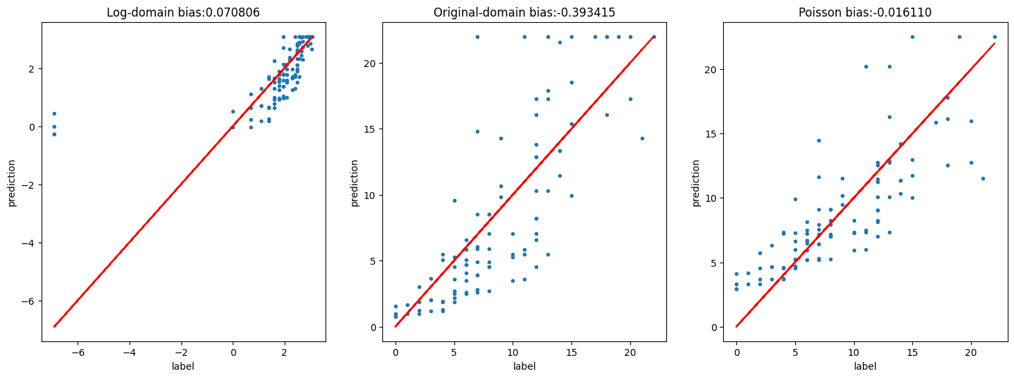
The first model predicts mean(log(label)) the second predicts log(mean(label)). Due to Jensen’s inequality, the first approach produces systematic negative bias

# Train log-transform model
training_samples = []
logz = np.log(0.001 + z)
vw = vowpalwabbit.Workspace(
    "-b 2 --loss_function squared -l 0.1 --holdout_off -f vw.log.model --readable_model vw.readable.log.model",
    quiet=True,
)
for i in range(len(logz)):
    training_samples.append(
        "{label} | x:{x} y:{y}".format(label=logz[i], x=x[i], y=y[i])
    )
# Do hundred passes over the data and store the model in vw.log.model
for iteration in range(100):
    for i in range(len(training_samples)):
        vw.learn(training_samples[i])
vw.finish()

# Generate predictions from the log-transform model
vw = vowpalwabbit.Workspace("-i vw.log.model -t", quiet=True)
log_predictions = [vw.predict(sample) for sample in training_samples]
# Measure bias in the log-domain
log_bias = np.mean(log_predictions - logz)
bias = np.mean(np.exp(log_predictions) - z)

Although the model is relatively unbiased in the log-domain where we trained our model, in the original domain there is underprediction as we expected from Jensenn’s inequality

# Train original domain model using poisson regression
training_samples = []
vw = vowpalwabbit.Workspace(
    "-b 2 --loss_function poisson -l 0.1 --holdout_off -f vw.poisson.model --readable_model vw.readable.poisson.model",
    quiet=True,
)
for i in range(len(z)):
    training_samples.append("{label} | x:{x} y:{y}".format(label=z[i], x=x[i], y=y[i]))
# Do hundred passes over the data and store the model in vw.log.model
for iteration in range(100):
    for i in range(len(training_samples)):
        vw.learn(training_samples[i])
vw.finish()

# Generate predictions from the poisson model
vw = vowpalwabbit.Workspace("-i vw.poisson.model", quiet=True)
poisson_predictions = [np.exp(vw.predict(sample)) for sample in training_samples]
poisson_bias = np.mean(poisson_predictions - z)

plt.figure(figsize=(18, 6))
# Measure bias in the log-domain
plt.subplot(131)
plt.plot(logz, log_predictions, ".")
plt.plot(logz, logz, "r")
plt.title("Log-domain bias:%f" % (log_bias))
plt.xlabel("label")
plt.ylabel("prediction")

plt.subplot(132)
plt.plot(z, np.exp(log_predictions), ".")
plt.plot(z, z, "r")
plt.title("Original-domain bias:%f" % (bias))
plt.xlabel("label")
plt.ylabel("prediction")

plt.subplot(133)
plt.plot(z, poisson_predictions, ".")
plt.plot(z, z, "r")
plt.title("Poisson bias:%f" % (poisson_bias))
plt.xlabel("label")
plt.ylabel("prediction")

Text(0, 0.5, 'prediction')